Why diversification fails during market crises…
Assume two variables, (x_1) and (x_2), follow generalized Wiener processes:
dx1 = a1·dt + b1·dz1 and dx2 = a2·dt + b2·dz2
The corresponding discrete–time versions of these continuous processes are:
Δx1=a1*Δt+b1*ε1* √Δt და Δx=a2*Δt+b2*ε2* √Δt
If we assume these processes are independent, then ε1 and ε2 are simply standard normal random variables, and the evolution can be simulated in the usual way (see Geometric Brownian Motion of Stock Price).
But if the random shocks are correlated, then their sampling must follow a bivariate normal distribution.
To sample from a bivariate or multivariate normal distribution we use the Cholesky decomposition.
In the bivariate case, the formula takes this familiar form:
Let ε1 = u. Then, to impose correlation:
ε2=ρ*u+√(1−ρ2) * v
where p is the correlation coefficient, and u and v are independent standard normal variables.
Below is a simulation of two stock price paths under different correlation assumptions:
- p = 0.9 (strong positive correlation)

- p = -0.9 (strong negative correlation)

- p = 0 (no correlation)

P.S.
Now let’s return to the question: Why does diversification fail during crises?
Because during a crisis the positive correlation between asset prices spikes dramatically.
It’s crucial to understand that correlation is not just a simple static coefficient between -1 and 1.
At a fundamental level, correlation between asset prices represents how much of one asset’s price shock is inherited by another asset’s price movement.
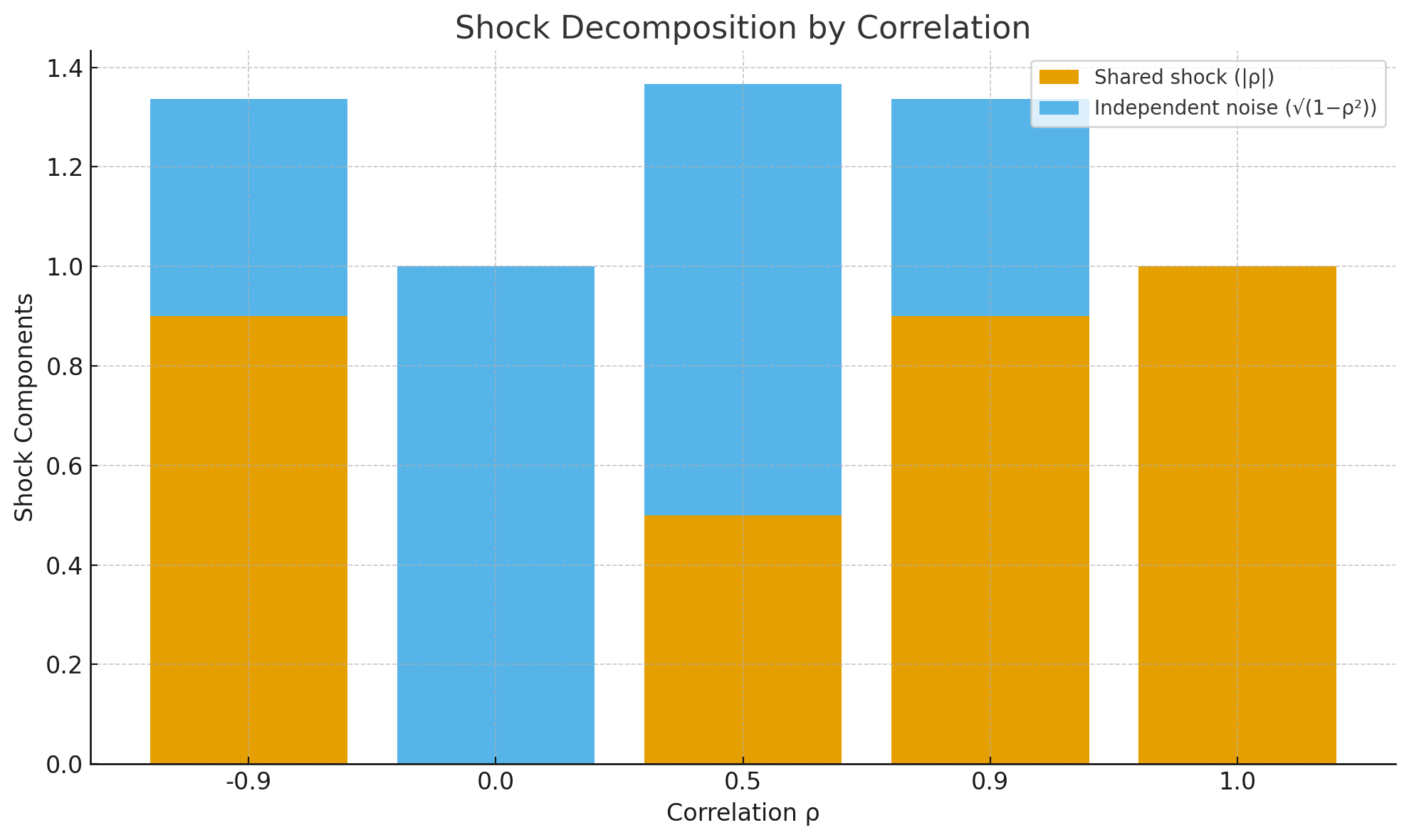
We can decompose the right side of the Cholesky sampling formula into two parts:
- Shock component: p* u
- Independent noise: √(1−ρ2) * v
This shows clearly that the influence of one asset’s shock on another depends directly on the correlation.
Below you can see a shock decomposition example for different correlation levels.

The attached Excel file contains a simulation of correlated asset price processes:
Source: Options, Futures & Other Derivatives, John C. Hull
Leave a Reply